
In this part of the TreeGen series, I’ll explain how I rendered the trees that were procedurally generated in the first part. Specifically, we’ll explore the advantages and challenges of using ray marching for rendering, my approach to implementing it, and the optimizations I applied to improve performance.
This post assumes some familiarity with ray marching and signed distance functions (SDFs). If you need a refresher, I highly recommend these excellent resources:
Why Use Ray Marching & Curves?
Typically, trees in 3D environments are rendered as mesh models made up of triangles using rasterization. Even if the branches are modeled as truncated cones, the end result is a complex mesh of polygons. TreeGen, however, takes a different approach: it converts branches into quadratic Bézier curves and renders them using ray marching. This method offers some advantages:
- Dynamic Shape Manipulation: Since the tree’s shape is represented mathematically as curves, you can dynamically alter it within the shader without needing to regenerate a mesh.
- Simpler Mathematical Representation: Instead of dealing with complex mesh generation and management, Bézier curves provide a clean, simple representation.
- Easier to Understand: Because everything is contained within the shader, and much of it is about mathematics, it is easier to understand and faster to experiment with.
However, the main disadvantage is that ray marching is generally slower than rasterization, especially for real-time rendering. Because of this, I had to optimize the ray marching code extensively.
Why Quadratic Bézier Curves?
I chose quadratic Bézier curves over truncated cones because they provide smoother results when rendering branches. For real-time performance, quadratic Bézier curves were preferable to cubic Bézier curves since their mathematical representation is simpler, and calculating their SDF is faster.
The main reason for choosing ray marching and Bézier curves, though, is that TreeGen is my thesis project. I wanted to experiment with non-traditional rendering techniques, and I found ray marching easier to work with for this purpose.
Although I’m presenting the final result here, I initially experimented with other methods such as line rendering, quad impostors, and ray marching truncated cones. Eventually, I settled on ray marching quadratic Bézier curves for the smoothest and most efficient results.
Quadratic Bézier Curve SDF
Bézier curves are parametric curves defined by two endpoints and one control point. TreeGen uses quadratic Bézier curves to render tree branches. While I’ll explain the mathematics behind its SDF, there are more detailed resources available for curves in general, such as this video by Freya Holmér.
The Quadratic Bézier Formula
Quadratic Bézier curves are defined by three points: the start point ($P_0$), the control point ($P_1$), and the end point ($P_2$). They are actually parabolas in 2D, which is handy. The curve is calculated using the formula:
$B(t) = (1 - t)^2P_0 + 2(1 - t)tP_1 + t^2P_2$
or
$B(t) = (P_0 - 2P_1 + P_2)t^2 + (P_1 - P_0)2t + P_0$
Where $t$ is a value between 0 and 1 representing the position along the curve.
Derivative of the Curve
The derivative of the curve is calculated by the formula:
$B’(t) = -2(1 - t)P_0 + 2(1 - 2t)P_1 + 2tP_2$
or
$B’(t) = 2(P_2 - 2P_1 + P_0)t + 2(P_1 - P_0)$
This derivative will help us find the closest point on the curve to any given point in space.
Substituting $A = P_1 - P_0$ and $B=P_2 - 2P_1 + P_0$:
$B(t) = Bt^2 + 2At + P_0$
$B’(t) = 2(Bt + A)$
Finding the Closest Point to the Curve
To find the closest point on the curve to a given point $P$, we need to solve the equation where the curve’s tangent is perpendicular to the vector between the curve and $P$. This is expressed as:
$B’(t).(P - B(t)) = 0$
Where $P$ is the given point and $.$ is the dot product. This can be rewritten as:
$(2(Bt + A)).(P - (Bt^2 + 2At + P_0)) = 0$
$(Bt + A).(P - Bt^2 - 2At - P_0) = 0$
Substitute $P’ = P_0 - P$:
$(Bt + A).-(Bt^2 + 2At + P’) = 0$
$B^2t^3+3ABt^2+(2A^2+BP’)t+AP’=0$
$t^3+\frac{3ABt^2+(2A^2+BP’)t+AP’}{B^2}=0$
This is a cubic equation, which can be solved using various methods. I will not go into detail on how it is solved. There are 3 possible solutions at max and the one that has the smallest distance to the given point is chosen.
Once the correct $t$ value is found, we can compute the distance to the curve’s offset surface, which is defined by a radius that varies along the curve:
$r(t) = r_{low} * (1-t) + r_{high}*t$
Where $r_{low}$ is the radius at the start of the curve and $r_{high}$ is the radius at the end. Finally, the distance from the point to the curve’s surface is given by:
This radius can be also eased based on $t$ to make the transition smoother, but I tried it and didn’t find it necessary.
Finally, the distance from the point to the curve’s surface is given by:
$d = |B(t) - P| - r(t)$
GLSL Code
Here’s the GLSL function that calculates the distance to a quadratic Bézier curve and finds the closest point:
vec2 sdBezier(vec3 p, Bezier bezier)
{
    vec3 A = bezier.start;
    vec3 B = bezier.mid;
    vec3 C = bezier.end;
    vec3 a = B - A;
    vec3 b = A - B * 2.0 + C;
    vec3 c = a * 2.0;
    vec3 d = A - p;

    vec3 k = vec3(3.*dot(a,b),2.*dot(a,a)+dot(d,b),dot(d,a)) / dot(b,b);


    vec2 t = solveCubic(k.x, k.y, k.z);
    vec2 clampedT = clamp(t, 0.0, 1.0);

    vec3 pos = A + (c + b * clampedT.x) * clampedT.x;
    float tt = t.x;
    float dis = length(pos - p);
    pos = A + (c + b * clampedT.y) * clampedT.y;
    float dis2 = length(pos - p);
    bool y = dis2 < dis;
    dis = mix(dis, dis2, y);
    tt = mix(t.x, t.y, y);
    //pos = A + (c + b*t.z)*t.z;
    //dis = min(dis, length(pos - p));
    return vec2(dis, tt);
}

vec2 dist(in vec3 pos, in Bezier bezier) {
    vec2 sdBranch = sdBezier(pos, bezier);

    float clampedT = clamp(sdBranch.y, 0.0, 1.0);
    float midDist = sdBranch.x - (1. - t) * bezier.lowRadius - t * bezier.highRadius;
    return vec2(midDist, sdBranch.y);
}
Notice that I do not return the clamped $t$ value, this is because I will use the $t$ value to check if the point is inside the curve or not.
To solve the cubic equation, we use this function:
vec2 solveCubic(float a, float b, float c) {
	// Depress the cubic to solve it
    float p = b - a*a / 3.0, p3 = p*p*p;
    float q = a * (2.0*a*a - 9.0*b) / 27.0 + c;
    float d = q*q + 4.0*p3 / 27.0;
    float offset = -a / 3.0;
    // One real root
    if(d >= 0.0) {
        // Cardano's method
        float z = sqrt(d);
        vec2 x = (vec2(z, -z) - q) / 2.0;
        vec2 uv = sign(x)*pow(abs(x), vec2(1.0/3.0));
        return vec2(offset + uv.x + uv.y);
    }
    // Three real roots
    // Trigonometric solution
    // x = 3q / 2p * sqrt(-3 / p)
    float x = -sqrt(-27.0 / p3) * q / 2.0;

    // This is an approximation for m=cos(acos(x)/3.0)
    x = sqrt(0.5+0.5*x);
    float m = x*(x*(x*(x*-0.008978+0.039075)-0.107071)+0.576974)+0.5;

    float n = sqrt(1.-m*m)*sqrt(3.);
    return vec2(m + m, -n - m) * sqrt(-p / 3.0) + offset;
}
Both of these functions are adapted from Inigo Quilez’s Quadratic Bezier distance shader.
Creating Curves from Branches
Hybrid Rendering
TreeGen employs a hybrid rendering approach: the tree body is rendered using ray marching, while simpler objects like leaves are rendered using rasterization. This is because ray marching, although flexible, is slower compared to rasterization. Rasterization works better for simple quads/meshes, making it ideal for leaves. I will explain the ray marching setup and how I matched the depth for both rendering techniques.
Ray Marching Setup
Ray marching is typically done on a full-screen quad, but in TreeGen, the ray marching shader operates per bounding box of each branch. This approach minimizes missed rays and optimizes performance. I used a simple axis-aligned bounding box (AABB) for the curves, although a tighter bounding object, like cylinders, might yield better performance. Bounding box calculations are done on the CPU using the methods from Inigo Quilez’s Bézier bounding box article and passed to the vertex shader. Once a pixel is rasterized, the fragment shader begins ray marching from the world-space position of the pixel along the following direction:
vec3 rayDir = normalize(worldPos - cameraDir);
Initially, I used fixed step count and minimum distance values, but I later optimized the process by adapting these parameters based on the distance between the camera and the bounding box. A curve that’s farther from the camera doesn’t need to be rendered with high detail, allowing for lower step counts and higher minimum distances, especially useful in shadow rendering.
Since the ray marching is confined to a bounding box, performing ray-marched boolean operations between curves is challenging. Instead, I handle continuity issues of sequential curves by adjusting control points and blending normals at curve endpoints. This improves the visual smoothness of sequential curves, although it doesn’t address discontinuities at branch points. I will explain how normal blending works later.
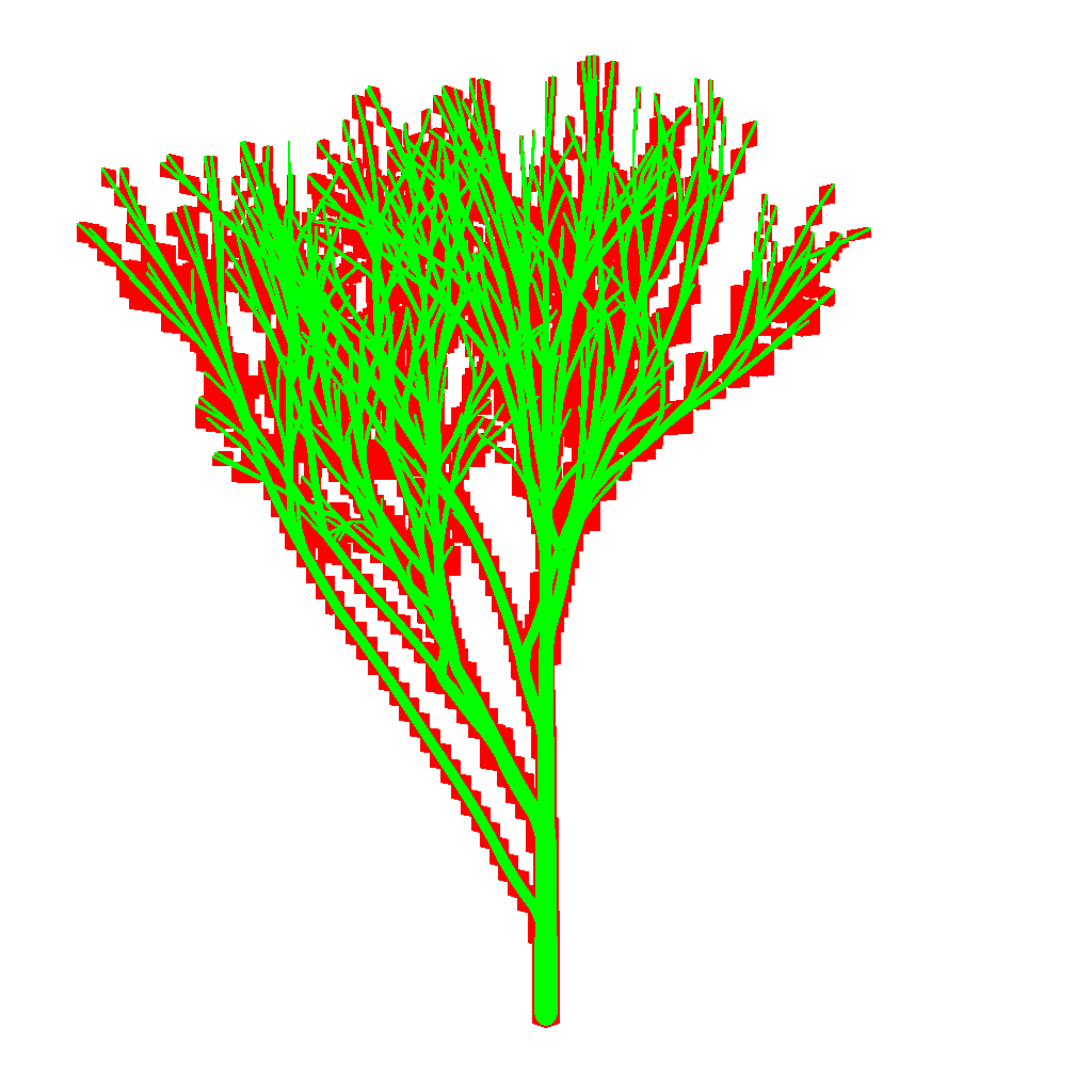
Below is a debug render demonstrating the ray marching setup & hit/miss rays with AABBs, it should also give some intuition on how the ray marching setup works:
C++ Code for Converting Branches to Curves
This function is rather long, so I’ll break it down into three parts. The first part calculates the control points of a Bézier curve based on the current branch, the previous branch, and the next branch:
void Branch::CalculateControlPoints(float curviness)
{
	const TreeNode& node = *from;
	TreeNode* dominantChild = from->dominantChild();
	length = node.length;
	if (node.order > 0 && node.parent->dominantChild()->id != node.id)
	{
		length += node.parent->length;
		bez.A = node.parent->startPos;
		bez.B = node.startPos + node.direction * node.length * 0.5f;
	}
	else
	{
		bez.A = node.startPos;
		vec3 parentPoint(0.0);

		if (node.order == 0)
			parentPoint = node.startPos + node.direction * node.length * 0.5f;
		else
			parentPoint = node.startPos + node.parent->direction * node.length * 0.5f;

		vec3 childPoint(0.0);
		if (dominantChild != nullptr)
			childPoint = node.endPos() - dominantChild->direction * node.length * 0.5f;
		else
			childPoint = node.startPos + node.direction * node.length * 0.5f;

		bez.B = (parentPoint + childPoint) / 2.0f;
	}
	bez.C = node.endPos();
	bez.B = glm::mix((bez.A + bez.C) / 2.0f, bez.B, curviness);

	float dots = glm::dot(glm::normalize(bez.B - bez.A), glm::normalize(bez.C - bez.A));

	if (glm::abs(dots) >= 0.9999f)
	{
		vec3 randomDir(1.0f, 0.0f, 0.0f);
		if (glm::abs(glm::dot(randomDir, glm::normalize(bez.C - bez.A)) >= 0.99))
			randomDir = vec3(0.0f, 1.0f, 0.0f);
		bez.B += glm::normalize(glm::cross(randomDir, bez.C - bez.A)) * 0.00005f;
	}
}
This function first checks whether the current branch is the dominant child (the thicker child branch) of its parent. If so, it will be rendered as a continuation of the parent’s curve.
If it is not the dominant child, the function makes the branch curve in its own direction smoothly. Control point $A$ is set to the parent’s start position, ensuring smooth branching. Control point $B$ is calculated as the midpoint between the branch’s start and end positions, and control point $C$ is set to the branch’s end position.
If the branch is dominant, $A$ is set to the branch’s start, and $B$ is blended between the parent’s and child’s continuations to ensure a smooth transition. $C$ is set to the branch’s end position.
Based on $curviness$ parameter, control point $B$ is blended between the midpoint of $A$ and $C$ and the calculated position. This is to make the curve smoother or more like a straight line.
Lastly, the function checks if the control points are colinear, if they are, then the distance function does not work correctly, so $B$ is offset slightly to make the control points not colinear.
The second part calculates the bounding box for the Bézier curve based on Inigo Quilez’s Bézier bounding box method:
void Branch::CalculateBoundingBox()
{
	// extremes
	vec3 mi = glm::min(bez.A, bez.C);
	vec3 ma = glm::max(bez.A, bez.C);


	mi -= bez.startRadius;
	ma += bez.startRadius;

	// maxima/minima point, if p1 is outside the current bbox/hull
	if (bez.B.x<mi.x || bez.B.x>ma.x || bez.B.y<mi.y ||
		bez.B.y>ma.y || bez.B.z < mi.x || bez.B.z > mi.y)
	{

		vec3 t = glm::clamp((bez.A - bez.B) / (bez.A - 2.0f * bez.B + bez.C), 0.0f, 1.0f);
		vec3 s = 1.0f - t;
		vec3 q = s * s * bez.A + 2.0f * s * t * bez.B + t * t * bez.C;

		mi = min(mi, q - bez.startRadius);
		ma = max(ma, q + bez.startRadius);
	}


	boundingBox = { mi, ma };
}
The final part of the function calculates UV offsets based on the lengths of successive branches:
void Branch::CalculateUVOffsets(float startLength, const vec3& lastPlaneNormal, float lastXOffset)
{
	// This is simple, y offset is based on the length of the curve sequence so far
	yOffset = startLength;
	// x offset is based on the angle between the last plane normal and the current plane normal
	bez.bezierPlaneNormal = normalize(glm::cross(bez.B - bez.A, bez.C - bez.A));

	vec3 bezDir = bez.evaluateDir(0.0f);

	// Normal of bezier curve on the plane defined by the curve
	vec3 bezierNormalOnPlane = glm::normalize(glm::cross(bez.bezierPlaneNormal, bezDir));

	// Angle between the last plane normal and the current plane normal
	float angle = glm::atan(glm::dot(bezierNormalOnPlane, lastPlaneNormal), glm::dot(bez.bezierPlaneNormal, lastPlaneNormal));

	xOffset = lastXOffset + angle;
}
Calculating Y offset is rather simple—it’s just the length of the curve sequence so far.
Calculating the X offset is trickier, and the process is similar in the shader. Here’s the code for both:
float calc_uvx(Branch branch, float clampedT, vec3 curPos) {
    Bezier curve = toBezier(branch);
    vec3 bezierPos = bezier(curve, clampedT);
    vec3 bezierPlaneNormal = normalize(cross(curve.mid - curve.start, curve.end - curve.start));
    vec3 bezierDir = normalize(bezier_dx(curve, clampedT));
    vec3 bezierNormalOnPlane = normalize(cross(bezierPlaneNormal,bezierDir));
    vec2 v = vec2(dot(curPos-bezierPos,bezierNormalOnPlane),dot(curPos-bezierPos,bezierPlaneNormal));

    return atan(v.y,v.x) + branch.uvOffset.x;
}
In the shader, it is calculated based on the curve’s plane normal and the normal of the curve on the plane. The plane’s normal is calculated simply as cross(B-A, C-A), and the normal of the curve on the plane is calculated as cross(planeNormal, curveDirection), where curveDirection is the derivative of the curve at $t$. Then, we get the coordinates on the basis with dot products and then calculate the angle using $atan$ function, lastly, we add the previous X offset to the angle. This is the same for calculating the offset from the previous branch, but the previous branch’s plane normal is used instead of $curPos-bezierPos$ that is used in the shader.
Note that using atan2 or acos will result in discontinuities, since they return in the range $[-\pi/2, \pi/2]$ or $[0, \pi]$ respectively, so atan, which returns in the range $[-\pi, \pi]$, is used. This also gets rid of the hack in Inigo Quilez’s shader, which uses acos for curve-to-curve and multiplies the offset by $-1$ for some curve indices.
Here is a 3D visualization of the UV offset calculation I made on Desmos.
Since ray marching is limited by the amount of steps, some bugs can occur, such as the ray terminating before hitting the curve with grazing angles & low step counts, here is an image demonstrating the problem:
I did not solve this problem in the project, but I suppose it could be solved by increasing the max step count if the direction of the ray is almost parallel to the curve direction.
Matching Depth
Since ray marching calculates the intersection point in world space, we need to convert the depth to screen space and perform perspective division.
Here’s how the process works:
- We need some properties of the camera, the ray direction, and hit depth from ray marching. I calculated the ray direction as the normalized vector from the camera position to a point on the transformed bounding box, which was rasterized.
float hitDepth;
vec3 rayDir;
vec3 cameraDir;
float farPlane;
float nearPlane;
- Convert the hit depth to eye space:
float eyeHitZ = -hitDepth * dot(cameraDir, rayDir);
- Convert the eye space depth to clip space:
float clipZ = ((farPlane + nearPlane) / (farPlane - nearPlane)) * eyeHitZ + [2.0 * farPlane * nearPlane / (farPlane - nearPlane)];
float clipW = -eyeHitZ;
- Perspective division, which will convert the clip space depth to normalized device coordinates (NDC):
float ndcDepth = clipZ / clipW;
// This is the same but in one line
float ndcDepth = ((farPlane + nearPlane) + (2.0 * farPlane * nearPlane) / eyeHitZ) / (farPlane - nearPlane);
- To write it into the depth buffer, we will need to convert it to the range $[0, 1]$. OpenGL exposes 3 variables for depth range:
gl_DepthRange.near,gl_DepthRange.far, andgl_DepthRange.diff, which are respectively $0.0$, $1.0$ and $1.0$ unless specified otherwise withglDepthRange(float nearVal, float farVal). Finally, we can calculate the value that will be written in the depth buffer as:
float depthBufferVal = ((gl_DepthRange.diff * ndcDepth) + gl_DepthRange.near + gl_DepthRange.far) / 2.0;
By default, gl_FragDepth is not an output of the fragment shader, if a shader writes to it, then it must be specified explicitly:
layout out float gl_FragDepth;
Writing the depth value to the depth buffer:
gl_FragDepth = depthBufferVal;
Since I use a bounding box and start the ray marching from its boundary, it is guaranteed that the calculated depth value will be bigger than the current depth value of the rasterized pixel, which was calculated from the bounding box. Because of this, I can mark the gl_FragDepth as (depth_greater) to theoretically enable early depth testing, which discards the fragment if the depth value is greater than the current depth value in the depth buffer, which was calculated previously from the result of another fragment shader. I say theoretically since I tested it in 3 different setups and it did not enable early depth testing, so I am not sure if it works or not. There is layout(early_fragment_tests) in; which forces early depth testing, but it disables depth writes in the fragment shader, which should not be the case since gl_FragDepth is marked as (depth_greater), and discard does not seem to work with it, so I cannot use it either.
Tree Shader
Data Structures
These are rather simple data structures, so I will not explain them in detail.
Branch data structure for static shader:
struct BranchData {
    mat4 model;
	vec4 start;
    vec4 mid;
	vec4 end;
    vec4 color;
	float lowRadius;
	float highRadius;
    float startLength;
    float branchLength;
    float uvOffset;
    int order;
};
modelis the model matrix of the branchstart,mid, andendare the control points of the Bézier curvecoloris the color of the branch that is used for debugginglowRadiusis the start radius,highRadiusis the end radius, note thatlowRadiusis bigger thanhighRadiusstartLengthis the length of the curve sequence so farbranchLengthis the length of the current curveuvOffsetis the X offset of the branchorderis the order of the branch in the tree, which is used for coloring the older branches darker.
Each curve/branch is a cube that is drawn using instancing, so BranchData is stored in an SSBO and accessed using the gl_InstanceID in the shaders.
For animated shader, I use a slightly different data structure:
// This is stored in the SSBO
struct AnimatedBranchData {
    mat4 model;
	vec4 start;
    vec4 mid;
	vec4 end;
    vec4 color;
	vec2 lowRadiusBounds;
	vec2 highRadiusBounds;
    vec2 TBounds;
    vec2 animationBounds;
    float startLength;
    float branchLength;
    float uvOffset;
    int order;
};

// This is the branch at a particular parameter t
struct AnimatedBranch {
    mat4 model;
    float endT;
	vec3 start;
    vec3 mid;
	vec3 end;
    vec3 color;
	float lowRadius;
	float highRadius;
    float startLength;
    float branchLength;
    float uvOffset;
    int order;
};
This structure is similar to the static branch data, but it has ranges for the radius and $t$. I will explain it further in the animated shader section.
Vertex Shader
This is a simple vertex shader that transforms vertices based on the model matrix on the AABB. Additionally, I inverted the bounding box if the camera is inside, so trees can be rendered from the inside while face culling is still enabled.
void main()
{
    mat4 model = branchs[gl_InstanceID].model;

    vec3 camPos = cam.pos_near.xyz;


    vec3 pos = model[3].xyz;
    vec3 dif = abs(camPos-pos);
    vec3 scale = vec3(model[0][0], model[1][1], model[2][2]);
    bool inside = min(dif, abs(scale) / 2.0) == dif;
    vec3 p = aPos * (float(!inside) * 2.0 - 1.0);

    vec4 calcP = model * vec4(p, 1.0);

    gl_Position = cam.vp * calcP;
    fragPos = calcP.xyz;

    instanceID = gl_InstanceID;
}
Static Fragment Shader
The static fragment shader performs the ray marching. I’ll break down the steps since the shader code is long and most of the techniques are already explained.
- Get the ray direction from
fragPos - cameraPosand normalize it. - Calculate the distance from the starting point to the bounding box, which helps determine the minimum distance and step count.
- Use the
sdBezierfunction in a ray marching loop to find the intersection point and the curve normal. - If the ray doesn’t hit the curve, discard the fragment.
- Calculate the UV coordinates for the hit point on the curve.
- Blend normals near the curve’s endpoints to smooth transitions between sequential curves (further explanation in blending normals).
- Calculate the depth value, if the intersecting point’s spline parameter $t$ is less than 0.0 or greater than 1.0, then it is on the spheres that are on the endpoints of the curve. Normally, this shouldn’t be a problem, but since sequential curves are not perfectly matched, spheres at the endpoints poke out of the previous/next branch, so I fixed it by offsetting the depth value by a small amount if the point is on the sphere. Then convert the depth value & write it to the depth buffer.
- Get the albedo color & normal of the point using the UV coordinates & textures. Then calculate the final normal using bump mapping.
- Calculate the lighting using the Blinn-Phong lighting model.
- Perform shadow mapping and percentage-closer filtering (PCF) to check for shadows.
- Output the final color.
The source code for this file can be found in the GitHub repository.
Blending Normals
Normals at the connection points of sequential curves don’t match perfectly, which causes a visible seam. To fix this, I assume that two curves are connected by a truncated cone. The cone’s bottom radius is the radius of the previous curve at $1-t_{normalBlend}$, and the top radius is the radius of the next curve at $t_{normalBlend}$. If a ray-marched point is outside the range $[t_{normalBlend}, 1-t_{normalBlend}]$, I blend it with the cone’s normal at the start/end, making the transition smoother.
I won’t go into detail on how the cone’s normal is calculated, but you can explore a 3D visualization I made on Desmos.
GLSL Code
vec3 coneNormal(in vec3 pos, in float t, in vec3 A, in vec3 B, in float Arad, in float Brad) {
    vec3 AP = normalize(pos-A);
    vec3 BP = normalize(pos-B);
    vec3 AB = normalize(B-A);
    vec3 Acone = normalize(AP - dot(AB, AP) * AB) * Arad + A;
    vec3 Bcone = normalize(BP - dot(AB, BP) * AB) * Brad + B;

    vec3 coneDif = normalize(Bcone-Acone);

    return normalize(AP - dot(AP, coneDif) * coneDif);
}
Animated Growth & Shader

Animating is rather simple with the ray marching setup I have, I simply interpolate the control points & radii of the curve based on the animation parameter $t$. The first step of the shader is calculating the interpolated points & radii, then the remaining steps are the same as the static shader.
Conclusion
In conclusion, I’m satisfied with the ray marching results, especially the ability to animate growth dynamically. The final output is good, although I think a more advanced lighting model would enhance it further. Through this project, I learned a great deal about OpenGL, ray marching, working with curves, and performance benchmarking (particularly with NSight).
If I had more time, I’d explore additional optimizations, different lighting models, and more dynamic manipulation of tree shapes. Below are the performance benchmarks for the ray marching shader using an RTX 2060:
| Figure | Branches | Total | Shaded Branches | Shaded Leaves | Branch Shadows | Leaf Shadows |
|---|---|---|---|---|---|---|
| Only Branches | 2,410 | 0.35ms | 0.35ms | - | - | - |
| Single Tree | 2,410 | 0.50ms | 0.29ms | 0.11ms | 0.06ms | 0.03ms |
| Forest | 237,551 | 12.0ms | 4.09ms | 3.90ms | 2.98ms | 1.02ms |
Thank you for reading! If you have any questions or feedback, feel free to comment.