What is this series about?
This series explores TreeGen, a project dedicated to the procedural generation and real-time rendering of trees. It was my bachelor’s thesis, which was developed over the course of a year. The series is divided into two main parts:
Tree Generation: This part is dedicated to the explanation of the self-organizing trees algorithm as outlined in the paper Self-organizing tree models for image synthesis by Pałubicki et al. I’ll break down the algorithm step-by-step and explain my approach to implementing it.
Tree Rendering: In the second part, I’ll cover the rendering techniques I have developed, which utilize ray marching quadratic Bézier curves.
You can find the project on Github and the thesis here. The project is written in C++20 and uses OpenGL 4.6 for rendering. When I wrote the project, I had little C++ experience, so the code might not be the best, sorry in advance.
This series not only showcases a practical application of procedural generation but also highlights the intricacies and challenges of real-time rendering.
Introduction to Procedural Tree Generation
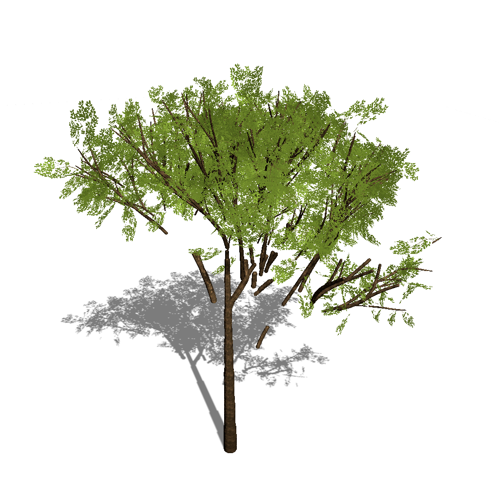
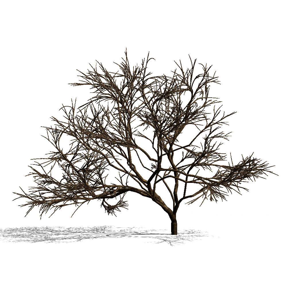
Procedural tree generation is essential in games and any type of VFX due to the complexity of manually creating trees with their intricate branching structures. This technique automates the creation process, enabling artists to quickly and efficiently produce a diverse range of trees. It’s particularly useful for generating forests, where a large number of unique trees are needed, saving both time and effort.
Procedural tree generation algorithms generally fall into two categories:
Fractal-Based Algorithms: These algorithms use recursive patterns to generate tree structures. While they are quick and straightforward to implement, they often neglect environmental factors. This can lead to unrealistic results, such as intersecting branches or implausible tree shapes.
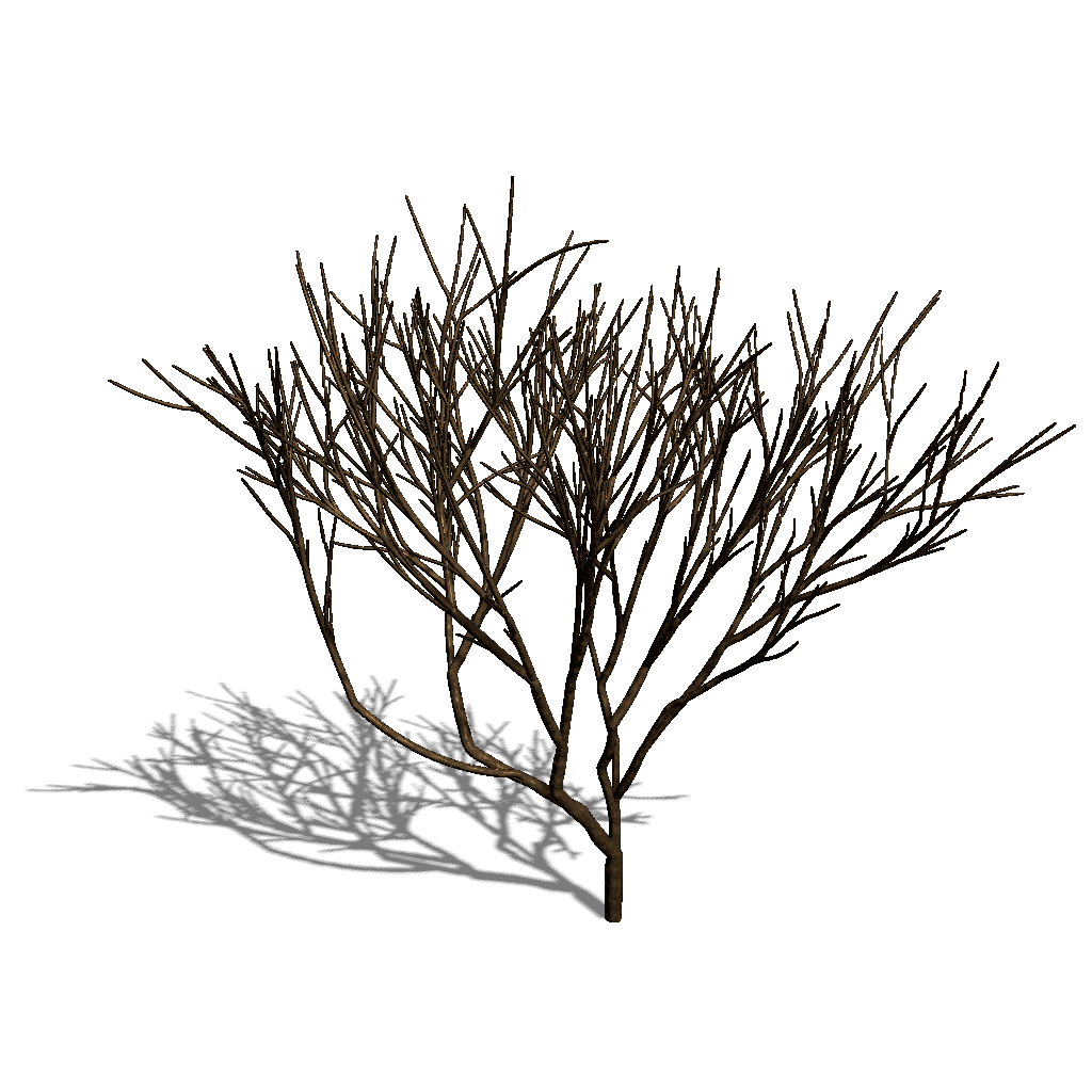
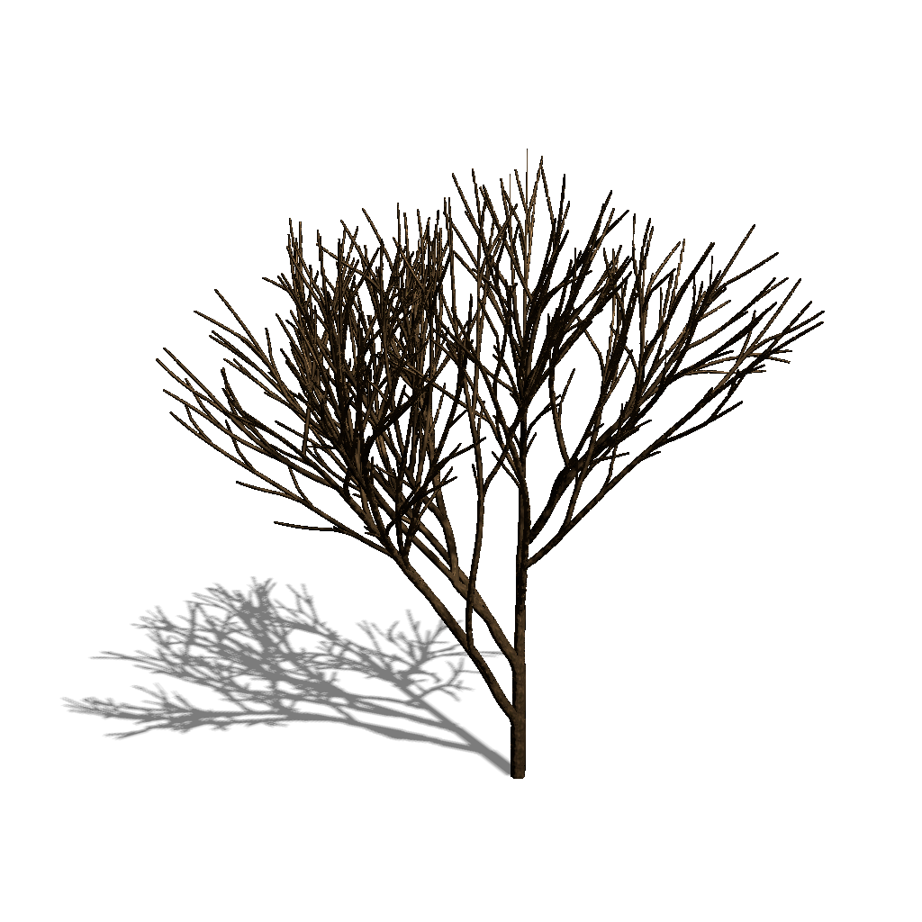
Self-Organizing Algorithms: In contrast, self-organizing algorithms model trees as dynamic systems where different parts of the tree compete for resources. This approach leads to more natural and non-intersecting tree structures, as it incorporates environmental factors and resource allocation.
For my project, I focused on real-time generation and reproducibility. Consequently, I chose the self-organizing tree model for its ability to produce more realistic and varied results. In the subsequent sections, I will discuss optimizations and techniques for achieving reproducible randomness in the tree generation process.
Overview of the Algorithm
A tree is represented as a recursive structure of connected branches. Each branch has a terminal (main) and a lateral bud, where each leaf bud can generate a new branch. This is an iterative algorithm where each iteration is divided into 5 steps, and I added another step to produce offspring trees:
- Calculating Light Received: Calculating how much light each leaf bud receives based on local environmental factors, and accumulate the light recursively summing up to the root.
- Distributing Growth Resources: Determine how much of the total resource is distributed to each bud.
- Growing New Branches: For each leaf bud with sufficient vigor, create new branches based on optimal direction and tropism vectors.
- Shedding Branches: Remove buds that do not receive enough resources (This step is optional).
- Calculating Branch Width: Calculate the branch width based on child count.
- Generating Offspring Trees: Introduce new trees around the parent tree to simulate seed dispersal and forest growth.
TreeNode struct for my implementation:
struct TreeNode
{
  enum NodeStatus
  {
    BUD, ALIVE, DEAD,
  };
  vec3 startPos;
  vec3 direction;
  float length = 1.0f;

  uint32 childCount = 0;

  uint8 nodeStatus = NodeStatus::BUD;
  TreeNodeId id = 0;
  uint32 order = 0;
  uint32 createdAt = 0;

  //iteration parameters
  float light = 0.0f;
  float vigor = 0.0f;

  //root if null
  TreeNode* parent;
  TreeNode* mainChild = nullptr;
  TreeNode* lateralChild = nullptr;
}
- Each node has a start position, direction and length. Start position is simply the same as the end position of its parent, which is calculated simply as
position + direction * length. childCountvariable keeps track of how many children each branch has, it is used while the shedding step and also to calculate the branch width.nodeStatusfield keeps track if a node leaf bud, a developed branch or a branch that was removed in the shedding step.orderis the distance of the node to the root node.createdAtis the iteration step that this node was created at.lightfield is calculated on step 1 as follows: If the node is a bud, then it is calculated as how much light the node receives, if the node is not a bud, then it is the sum of how much light its children receive.- Similar to
light,vigoris the growth resource that was distributed to a node from its parent, it is used to determine if a leaf node should produce new branches, or if a bud should shed.
Step 1: Calculating Light Received
This step is implemented as a recursive function starting from the root, accumulating light received by leaf buds. While accumulating the light, each node must remember how much light it receives in total from its children or from the environment, since it will be used to determine the distribution of growth resources in step 2.
C++ Implementation
float Tree::accumulateLightRecursive(TreeNode& node)
{
	if (node.nodeStatus == TreeNode::BUD)
	{
		if (!world->isOutOfBounds(node.startPos))
		{
			node.light = lightAtBud(node);
		}
		else
		{
			node.light = 0.0f;
		}
	}
	else if (node.nodeStatus == TreeNode::ALIVE)
	{
		node.light = accumulateLightRecursive(*node.mainChild) + accumulateLightRecursive(*node.lateralChild);
	}
	else
	{
		node.light = 0.0f;
	}
	return node.light;
}
lightAtBud function can be implemented in many ways, it might be calculated from a shadow map, or even by ray tracing, or something that is not about light at all, it is just how much resource a bud receives. The paper proposes 2 methods: Space Colonization and Shadow Propagation. I implemented only the Shadow Propagation algorithm, but I will explain both.
Space Colonization
This method does not care about light, but it is solely based on buds competing to occupy more points that are distributed in the world. The points may be distributed randomly, or they might be created by a user that fills the world with points using a tool similar to a brush, resulting in more artistic control.
Each bud occupies the points that it is close to. Each leaf bud has a perception volume that is a cone in the direction of the bud, how much resource a bud has is calculated by how many unoccupied points the perception volume contains.
Shadow propagation
This method assumes a uniform light source that points downwards, and tries to calculated how much light each bud receives. The world is divided into voxels, where each voxel is used to determine how much light is blocked in a voxel. The buds cast pyramid like shadows downwards, starting from their position. The shadow has a height $q_{max}$, where each shadow in a cell is calculated as $a*b^{-q}$, where $q$ is the height difference between the cell and the bud’s cell. This is an accumulative calculation, so multiple buds casting shadows on a cell are summed, up to max $1.0$.
Note that both of these methods effects can be calculated in a global space, meaning that they are able to effect other trees, because of this, coupling multiple trees or generating a forest becomes trivial.
Step 2: Distributing Growth Resources
This is the almost the reverse of the first step, but the tree might decide to distribute the received light favoring the main childs or lateral childs, this is controlled by the apical control($\lambda$) parameter. The received light is multiplied by a parameter called vigorMultiplier, which is a parameter basically controlling how much trees grow.
Equations for Resource Distribution
The equations used to calculate the vigor for the main and lateral children are as follows:
$ tempVigor_{main} = \lambda * light_{main};$
$ tempVigor_{lateral} = (1 - \lambda) * light_{lateral};$
$ multiplier = \frac{vigor}{tempVigor_{main} + tempVigor_{lateral}}; $
$ vigor_{main} = tempVigor_{main} * multiplier; $
$ vigor_{lateral} = tempVigor_{lateral} * multiplier; $
C++ Implementation
void Tree::distributeVigorRecursive(TreeNode& node)
{
	if (node.nodeStatus != TreeNode::ALIVE)
		return;
	auto& growthData = getGrowthData();
	float apicalControl = growthData.apicalControl;
	float mainV = 0.0f;
	float lateralV = 0.0f;
	if (node.mainChild->nodeStatus != TreeNode::DEAD)
	{
		mainV = apicalControl * node.mainChild->light;
	}
	if (node.lateralChild->nodeStatus != TreeNode::DEAD)
	{
		lateralV = (1.0f - apicalControl) * node.lateralChild->light;
	}
	float tot = mainV + lateralV;
	if (tot == 0.0f)
		return;
	float multiplier = node.vigor / (tot);
	node.mainChild->vigor = mainV * multiplier;
	node.lateralChild->vigor = lateralV * multiplier;
	distributeVigorRecursive(*node.mainChild);
	distributeVigorRecursive(*node.lateralChild);
}
Apical Control
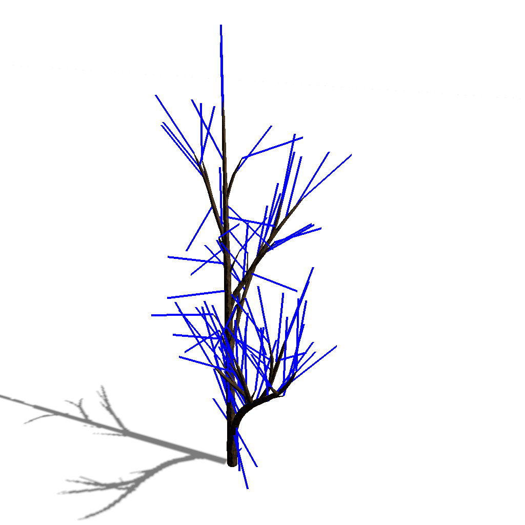
Step 3: Growing New Branches
In this step, new branches are generated from each leaf bud based on the amount of vigor and the direction vectors. The direction of new branches is influenced by the optimal direction and a tropism vector, simulating environmental effects like gravity or wind.
Optimal direction calculation is dependent on the method used in the light calculation step:
Space Colonization: The optimal direction is the average of vectors pointing to the unoccupied points in the perception volume.
Shadow Propagation: The optimal direction is the negative gradient of the shadow map, mostly resulting in a upwards direction, simulating the effect of sunlight.
The tropism vector is a vector that is added to the optimal direction, simulating the effect of wind or gravity.
C++ Implementation
void Tree::addShootsRecursive(TreeNode& node)
{
	if (node.nodeStatus == TreeNode::ALIVE)
	{
		addShootsRecursive(*node.mainChild);
		addShootsRecursive(*node.lateralChild);
		return;
	}
	else if (node.nodeStatus == TreeNode::DEAD)
	{
		return;
	}

	float vigor = node.vigor;
	int vigorFloored = static_cast<int>(glm::floor(vigor));

	auto& growthData = getGrowthData();
	float metamerLength = growthData.baseLength * vigor / glm::floor(vigor);

	if (world->isOutOfBounds(node.startPos))
		return;

	vec3 optimal = world->getOptimalDirection(node.startPos);

	vec3 direction = node.direction;

	TreeNode* current = &node;


	for (int i = 0; i < vigorFloored; i++)
	{
		if (world->isOutOfBounds(current->startPos))
			break;

		direction = glm::normalize(direction + growthData.directionWeights.x * optimal + growthData.directionWeights.y * growthData.tropism);
		current->length = metamerLength;
		current->direction = direction;
		budToMetamer(*current);
		current = current->mainChild;
	}
}

void Tree::budToMetamer(TreeNode& bud)
{
	bud.mainChild = new TreeNode(&bud, lastNodeId, bud.endPos(), bud.direction);
	lastNodeId++;
	vec3 lateralDir = util::randomPerturbateVector(glm::normalize(bud.direction), getGrowthData().lateralAngle, world->getWorldInfo().seed + seed + age + bud.id * 2 + 2);
	bud.lateralChild = new TreeNode(&bud, lastNodeId, bud.endPos(), lateralDir);
	budCount++;
	lastNodeId++;

	bud.nodeStatus = TreeNode::ALIVE;
	bud.createdAt = age;
	metamerCount++;
	maxOrder = glm::max(maxOrder, bud.order + 1);

	addShadows(*bud.mainChild);
}
Note that I do not give the id of the new nodes as $id_{main} = 2 * id_{parent}$ which was my first attempt, this results in overflow after 32 consecutive buds(uint32), which was a hard to detect problem when some trees were starting to miss some branches after a certain order due to id collisions.
The randomPerturbateVector function is based on this https://stackoverflow.com/a/2660181. It is used to add a randomness to the direction of the lateral branches and it is essential for simulating natural variability in branches of trees. Note that I pass seed and id as a parameter to the function, where I use it to generate a random value from a noise function, this ensures reproducability of the randomness.
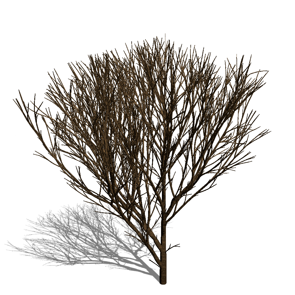
Step 4: Shedding Branches
In this step, the tree undergoes a pruning process to remove branches that are not receiving sufficient resources. This step simulates competition among branches and ensures that outdated branches are removed, resulting in a more realistic and healthy tree structure.
Shedding is crucial for simulating natural competition for resources and improving the realism of tree growth. By removing less competitive or outdated branches, the tree can better allocate resources to healthier and more promising branches. Also, this step ensures that branches that were grown when the tree was a sapling, but should not be present in the further iterations are removed, resulting in much more realistic trees.
C++ Implementation
void Tree::shedBranchsRecursive(TreeNode& node)
{
	if (node.nodeStatus != TreeNode::ALIVE)
		return;

	auto& growthData = getGrowthData();
	float p = node.vigor - growthData.shedMultiplier *
		glm::pow(glm::pow(node.childCount, 1.0f / growthData.radiusN), growthData.shedExp);

	if (age - node.createdAt < 4 || p >= 0)
	{
		shedBranchsRecursive(*node.mainChild);
		shedBranchsRecursive(*node.lateralChild);
		return;
	}

	node.nodeStatus = TreeNode::DEAD;
	cachedBranchs.erase(node.id);
	if (node.order != 0 && node.parent->mainChild->id == node.id)
	{
		removeShadows(node);
	}
	std::queue<TreeNode*> query({ node.mainChild, node.lateralChild });
	if (node.mainChild->nodeStatus != TreeNode::BUD)
	{
		removeShadows(*node.mainChild);
	}
	while (!query.empty())
	{
		TreeNode* sel = query.front();
		cachedBranchs.erase(sel->id);
		if (sel->nodeStatus == TreeNode::ALIVE)
		{
			query.emplace(sel->mainChild);
			if (sel->mainChild->nodeStatus != TreeNode::DEAD)
				removeShadows(*sel->mainChild);

			query.emplace(sel->lateralChild);
		}
		query.pop();
		delete sel;
	}
	node.mainChild = nullptr;
	node.lateralChild = nullptr;
}
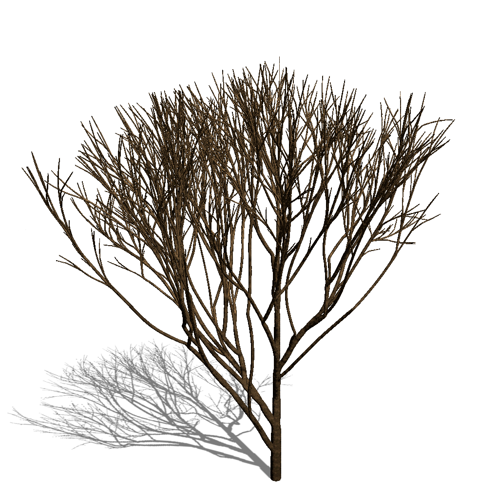
Step 5: Calculating Branch Width
Branch width is a crucial aspect of rendering trees, as it influences their appearance and realism. It is dependent on width of trees and calculated as:
$width^{radiusN} = width_{main}^{radiusN} + width_{lateral}^{radiusN}$
The radiusN parameter controls how much the width of the main and lateral branches affect the parent branch. In my implementation, I only calculate the child count of each bud, later I will use the child count to calculate branch width and distribute leaves, but since they only effect the render of the tree, I do not calculate them until I render the tree.
uint32 Tree::calculateChildCountRecursive(TreeNode& node)
{
	if (node.nodeStatus == TreeNode::BUD)
	{
		return 1;
	}
	else if (node.nodeStatus == TreeNode::DEAD)
	{
		return 1;
	}
	else
	{
		uint32 newChildCount = calculateChildCountRecursive(*node.mainChild) + calculateChildCountRecursive(*node.lateralChild);
		node.childCount = glm::max(node.childCount, newChildCount);
		return node.childCount;
	}
}
If a node is shed, its parent should not get smaller, so I keep the max child count of each node and use it if current child count is smaller.
Generating Leaves
Generating leaves involves using several parameters to ensure that the leaves are distributed and sized appropriately. This step primarily focuses on distributing leaves based on the characteristics of the branches.
Parameters
leafMaxChildCount: Specifies the maximum number of children a branch can have before it is considered a main branch and does not produce leaves.leafMinOrder: Defines the minimum branch order required before leaves can be generated. This prevents leaf generation on trees that are too young/small.leafDensity: Controls how densely leaves are distributed along the branch.leafSizeMultiplier: Adjusts the size of the leaves.
void Branch::generateLeaves(uint32 maxChildCount, uint32 minOrder, float leafDensity, float sizeMultiplier, bool forceRegen)
{
	if (minOrder > from->order)
	{
		leaves.clear();
		return;
	}
	TreeNode* dominantChild = from->dominantChild();
	uint32 domChildCount = dominantChild == nullptr ? 0 : dominantChild->childCount;
	if (dominantChild == nullptr)
	{
		dominantChild = nullptr;
	}
	if (domChildCount >= maxChildCount)
	{
		leaves.clear();
		return;
	}
	if (!forceRegen && !leaves.empty())
		return;
	leaves.clear();
	float chance = length * leafDensity;

	uint32 id = from->id;
	uint32 hashed = util::hash(id);
	for (int i = 0; i < glm::max(leafDensity, 5.0f); i++)
	{
		uint32 hashedI = util::hash(i);
		if ((util::IntNoise2D(hashed, hashedI) * 0.5f + 0.5f) < chance)
		{
			chance--;
		}
		else
		{
			break;
		}
		float t = util::IntNoise2D(id, i) * 0.5f + 0.5f;

		float rndAngle = PI * util::IntNoise2D(hashed, i);

		float size = sizeMultiplier * (util::IntNoise2D(id, hashedI) * 0.3f + 0.7f);

		if (t > 0.9)
		{
			size *= 1.0f;
		}

		leaves.emplace_back(this, t, size, rndAngle);
	}
}
Similar to the lateral bud direction, I use a hash & noise functions to generate a random value, this ensures reproducability of the randomness.
Step 6: Generating Offspring Trees
This step is not in the original algorithm, but it is rather simple, if a tree has enough vigor and has aged enough, then some new trees are generated close to the tree. This is used to simulate the effect of a tree dropping seeds, and new trees growing around the parent tree, which results in a forest. Also, this makes the trees compete with each other, since stronger trees will survive and produce offspring trees while weaker trees will die(from shedding). This can be also extended into a breeding/mutation system, where offspring trees have a chance to mutate, resulting in different trees, and evolution of the forest, though I did not implement this feature.
New tree count & max distance is calculated based on $log(vigor_{root})$.
Optimizations & Benchmarking
Profiling revealed that the majority of computation time was spent on adding and removing shadows in the shadow map. Here’s a summary of the key optimizations:
Look-up Table for Shadow Map: Calculating the shadow value per cell in the shadow map was a bottleneck due to the
pow(float, float)operation. I implemented a look-up table to store the shadow map values, which significantly improved performance. This is only possible since there are only $q_{max}$ different values that can be calculated, so I pre-calculate them and store them in a look-up table.Keep results of previous iterations: At first I was calculating the shadow map for every bud in every iteration, I realized that the shadow map does not change much between iterations, so I only calculate the differences caused by new buds or removed buds, which resulted in a huge performance increase.
Deferred Leaf Generation: I have a feature that lets the user preview the result of the next $n$ iterations, so that they can change the parameters without effecting the current tree. This meant that I did not need to generate leaves/calculate branches for the in-between iterations, which is why I decoupled the leaf generation step from the main iteration loop.
Each step in the iterations can be parallalized, some papers even implement it in compute shader, but I did not have the time to implement it, though it is a good optimization to consider which I would like to explore in the future.
Benchmark Results
The following table summarizes the performance benchmarks of the final implementation:
| Branchs | Total | Light | Vigor | New Shoots | Shedding | |
|---|---|---|---|---|---|---|
| Single Tree | $2,410$ | $5.98ms$ | $1.06ms$ | $0.5ms$ | $3.95ms$ | $0.86ms$ |
| Two Trees | $3,497$ | $8.46ms$ | $1.56ms$ | $0.07ms$ | $5.37ms$ | $1.33ms$ |
| Forest | $237,551$ | $1402ms$ | $349.26ms$ | $14.88ms$ | $722.8ms$ | $377.2ms$ |
Conclusion
This post was about the self-organizing tree algorithm, and how I implemented it in my project TreeGen. This algorithm shows promise for generating various organic structures, and I look forward to exploring its potential further. In the next post, I’ll discuss the tree rendering techniques used in TreeGen. Feel free to leave questions or suggestions in the comments below.